This is documentation for an old release of NumPy (version 1.18). Read this page Search for this page in the documentation of the latest stable release (version 2.2).

numpy.random.power

numpy.random.power(a, size=None)

Draws samples in [0, 1] from a power distribution with positive exponent a - 1.

Also known as the power function distribution.

Note

New code should use the power method of a default_rng() instance instead; see random-quick-start.

Parameters

afloat or array_like of floats

Parameter of the distribution. Must be non-negative.

sizeint or tuple of ints, optional

Output shape. If the given shape is, e.g., (m, n, k), then m * n * k samples are drawn. If size is None (default), a single value is returned if a is a scalar. Otherwise, np.array(a).size samples are drawn.

Returns

outndarray or scalar

Drawn samples from the parameterized power distribution.

Raises

ValueError

If a < 1.

See also

Generator.power

which should be used for new code.

Notes

The probability density function is

The power function distribution is just the inverse of the Pareto distribution. It may also be seen as a special case of the Beta distribution.

It is used, for example, in modeling the over-reporting of insurance claims.

References

1

Christian Kleiber, Samuel Kotz, “Statistical size distributions in economics and actuarial sciences”, Wiley, 2003.

2

Heckert, N. A. and Filliben, James J. “NIST Handbook 148: Dataplot Reference Manual, Volume 2: Let Subcommands and Library Functions”, National Institute of Standards and Technology Handbook Series, June 2003. https://www.itl.nist.gov/div898/software/dataplot/refman2/auxillar/powpdf.pdf

Examples

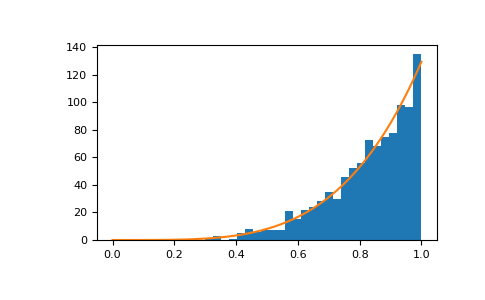
Draw samples from the distribution:

>>>

>>> a = 5. # shape
>>> samples = 1000
>>> s = np.random.power(a, samples)

Display the histogram of the samples, along with the probability density function:

>>>

>>> import matplotlib.pyplot as plt
>>> count, bins, ignored = plt.hist(s, bins=30)
>>> x = np.linspace(0, 1, 100)
>>> y = a*x**(a-1.)
>>> normed_y = samples*np.diff(bins)[0]*y
>>> plt.plot(x, normed_y)
>>> plt.show()

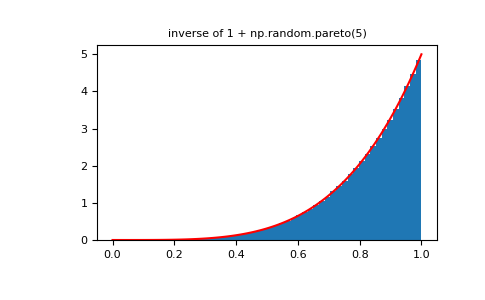
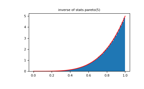
Compare the power function distribution to the inverse of the Pareto.

>>>

>>> from scipy import stats 
>>> rvs = np.random.power(5, 1000000)
>>> rvsp = np.random.pareto(5, 1000000)
>>> xx = np.linspace(0,1,100)
>>> powpdf = stats.powerlaw.pdf(xx,5)  

>>>

>>> plt.figure()
>>> plt.hist(rvs, bins=50, density=True)
>>> plt.plot(xx,powpdf,'r-')  
>>> plt.title('np.random.power(5)')

>>>

>>> plt.figure()
>>> plt.hist(1./(1.+rvsp), bins=50, density=True)
>>> plt.plot(xx,powpdf,'r-')  
>>> plt.title('inverse of 1 + np.random.pareto(5)')

>>>

>>> plt.figure()
>>> plt.hist(1./(1.+rvsp), bins=50, density=True)
>>> plt.plot(xx,powpdf,'r-')  
>>> plt.title('inverse of stats.pareto(5)')