numpy.percentile¶

numpy.percentile(a, q, axis=None, out=None, overwrite_input=False, method='linear', keepdims=False, *, interpolation=None)[source]¶

Compute the q-th percentile of the data along the specified axis.

Returns the q-th percentile(s) of the array elements.

Parameters

aarray_like

Input array or object that can be converted to an array.

qarray_like of float

Percentile or sequence of percentiles to compute, which must be between 0 and 100 inclusive.

axis{int, tuple of int, None}, optional

Axis or axes along which the percentiles are computed. The default is to compute the percentile(s) along a flattened version of the array.

Changed in version 1.9.0: A tuple of axes is supported

outndarray, optional

Alternative output array in which to place the result. It must have the same shape and buffer length as the expected output, but the type (of the output) will be cast if necessary.

overwrite_inputbool, optional

If True, then allow the input array a to be modified by intermediate calculations, to save memory. In this case, the contents of the input a after this function completes is undefined.

methodstr, optional

This parameter specifies the method to use for estimating the percentile. There are many different methods, some unique to NumPy. See the notes for explanation. The options sorted by their R type as summarized in the H&F paper [1] are:

‘inverted_cdf’
‘averaged_inverted_cdf’
‘closest_observation’
‘interpolated_inverted_cdf’
‘hazen’
‘weibull’
‘linear’ (default)
‘median_unbiased’
‘normal_unbiased’

The first three methods are discontiuous. NumPy further defines the following discontinuous variations of the default ‘linear’ (7.) option:

‘lower’
‘higher’,
‘midpoint’
‘nearest’

Changed in version 1.22.0: This argument was previously called “interpolation” and only offered the “linear” default and last four options.

keepdimsbool, optional

If this is set to True, the axes which are reduced are left in the result as dimensions with size one. With this option, the result will broadcast correctly against the original array a.

New in version 1.9.0.

interpolationstr, optional

Deprecated name for the method keyword argument.

Deprecated since version 1.22.0.

Returns

percentilescalar or ndarray: If q is a single percentile and axis=None, then the result is a scalar. If multiple percentiles are given, first axis of the result corresponds to the percentiles. The other axes are the axes that remain after the reduction of a. If the input contains integers or floats smaller than float64, the output data-type is float64. Otherwise, the output data-type is the same as that of the input. If out is specified, that array is returned instead.

See also

mean
median: equivalent to percentile(..., 50)
nanpercentile
quantile: equivalent to percentile, except q in the range [0, 1].

Notes

Given a vector V of length N, the q-th percentile of V is the value q/100 of the way from the minimum to the maximum in a sorted copy of V. The values and distances of the two nearest neighbors as well as the method parameter will determine the percentile if the normalized ranking does not match the location of q exactly. This function is the same as the median if q=50, the same as the minimum if q=0 and the same as the maximum if q=100.

This optional method parameter specifies the method to use when the desired quantile lies between two data points i < j. If g is the fractional part of the index surrounded by i and alpha and beta are correction constants modifying i and j.

Below, ‘q’ is the quantile value, ‘n’ is the sample size and alpha and beta are constants. The following formula gives an interpolation “i + g” of where the quantile would be in the sorted sample. With ‘i’ being the floor and ‘g’ the fractional part of the result.

\[i + g = (q - alpha) / ( n - alpha - beta + 1 )\]

The different methods then work as follows

inverted_cdf:: method 1 of H&F [1]. This method gives discontinuous results: * if g > 0 ; then take j * if g = 0 ; then take i
averaged_inverted_cdf:: method 2 of H&F [1]. This method give discontinuous results: * if g > 0 ; then take j * if g = 0 ; then average between bounds
closest_observation:: method 3 of H&F [1]. This method give discontinuous results: * if g > 0 ; then take j * if g = 0 and index is odd ; then take j * if g = 0 and index is even ; then take i
interpolated_inverted_cdf:: method 4 of H&F [1]. This method give continuous results using: * alpha = 0 * beta = 1
hazen:: method 5 of H&F [1]. This method give continuous results using: * alpha = 1/2 * beta = 1/2
weibull:: method 6 of H&F [1]. This method give continuous results using: * alpha = 0 * beta = 0
linear:: method 7 of H&F [1]. This method give continuous results using: * alpha = 1 * beta = 1
median_unbiased:: method 8 of H&F [1]. This method is probably the best method if the sample distribution function is unknown (see reference). This method give continuous results using: * alpha = 1/3 * beta = 1/3
normal_unbiased:: method 9 of H&F [1]. This method is probably the best method if the sample distribution function is known to be normal. This method give continuous results using: * alpha = 3/8 * beta = 3/8
lower:: NumPy method kept for backwards compatibility. Takes i as the interpolation point.
higher:: NumPy method kept for backwards compatibility. Takes j as the interpolation point.
nearest:: NumPy method kept for backwards compatibility. Takes i or j, whichever is nearest.
midpoint:: NumPy method kept for backwards compatibility. Uses (i + j) / 2.

References

1(1,2,3,4,5,6,7,8,9,10): R. J. Hyndman and Y. Fan, “Sample quantiles in statistical packages,” The American Statistician, 50(4), pp. 361-365, 1996

Examples

>>> a = np.array([[10, 7, 4], [3, 2, 1]])
>>> a
array([[10,  7,  4],
       [ 3,  2,  1]])
>>> np.percentile(a, 50)
3.5
>>> np.percentile(a, 50, axis=0)
array([6.5, 4.5, 2.5])
>>> np.percentile(a, 50, axis=1)
array([7.,  2.])
>>> np.percentile(a, 50, axis=1, keepdims=True)
array([[7.],
       [2.]])

>>> m = np.percentile(a, 50, axis=0)
>>> out = np.zeros_like(m)
>>> np.percentile(a, 50, axis=0, out=out)
array([6.5, 4.5, 2.5])
>>> m
array([6.5, 4.5, 2.5])

>>> b = a.copy()
>>> np.percentile(b, 50, axis=1, overwrite_input=True)
array([7.,  2.])
>>> assert not np.all(a == b)

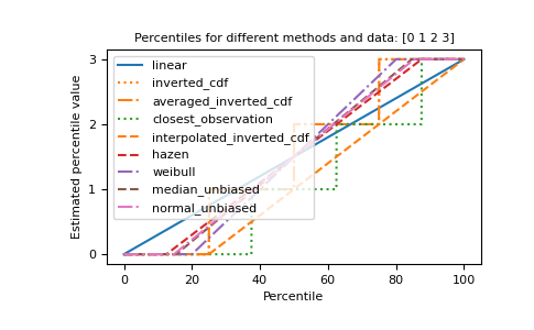
The different methods can be visualized graphically:

import matplotlib.pyplot as plt

a = np.arange(4)
p = np.linspace(0, 100, 6001)
ax = plt.gca()
lines = [
    ('linear', '-', 'C0'),
    ('inverted_cdf', ':', 'C1'),
    # Almost the same as `inverted_cdf`:
    ('averaged_inverted_cdf', '-.', 'C1'),
    ('closest_observation', ':', 'C2'),
    ('interpolated_inverted_cdf', '--', 'C1'),
    ('hazen', '--', 'C3'),
    ('weibull', '-.', 'C4'),
    ('median_unbiased', '--', 'C5'),
    ('normal_unbiased', '-.', 'C6'),
    ]
for method, style, color in lines:
    ax.plot(
        p, np.percentile(a, p, method=method),
        label=method, linestyle=style, color=color)
ax.set(
    title='Percentiles for different methods and data: ' + str(a),
    xlabel='Percentile',
    ylabel='Estimated percentile value',
    yticks=a)
ax.legend()
plt.show()

numpy.ptp

numpy.nanpercentile