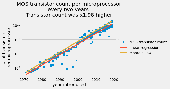
Determining Moore’s Law with real data in NumPy

Scatter plot of MOS transistor count per microprocessor every two years as a demonstration of Moore's Law.

The number of transistors reported per a given chip plotted on a log scale in the y axis with the date of introduction on the linear scale x-axis. The blue data points are from a transistor count table. The red line is an ordinary least squares prediction and the orange line is Moore’s law.

What you’ll do¶

In 1965, engineer Gordon Moore predicted that transistors on a chip would double every two years in the coming decade [1]. You’ll compare Moore’s prediction against actual transistor counts in the 53 years following his prediction. You will determine the best-fit constants to describe the exponential growth of transistors on semiconductors compared to Moore’s Law.

Skills you’ll learn¶

Load data from a *.csv file
Perform linear regression and predict exponential growth using ordinary least squares
You’ll compare exponential growth constants between models
Share your analysis in a file:
- as NumPy zipped files *.npz
- as a *.csv file
Assess the amazing progress semiconductor manufacturers have made in the last five decades

What you’ll need¶

1. These packages:

NumPy
Matplotlib

imported with the following commands

import matplotlib.pyplot as plt
import numpy as np

2. Since this is an exponential growth law you need a little background in doing math with natural logs and exponentials.

You’ll use these NumPy and Matplotlib functions:

np.loadtxt: this function loads text into a NumPy array
np.log: this function takes the natural log of all elements in a NumPy array
np.exp: this function takes the exponential of all elements in a NumPy array
lambda: this is a minimal function definition for creating a function model
plt.semilogy: this function will plot x-y data onto a figure with a linear x-axis and $\log_{10}$ y-axis plt.plot: this function will plot x-y data on linear axes
slicing arrays: view parts of the data loaded into the workspace, slice the arrays e.g. x[:10] for the first 10 values in the array, x
boolean array indexing: to view parts of the data that match a given condition use boolean operations to index an array
np.block: to combine arrays into 2D arrays
np.newaxis: to change a 1D vector to a row or column vector
np.savez and np.savetxt: these two functions will save your arrays in zipped array format and text, respectively

Building Moore’s law as an exponential function¶

Your empirical model assumes that the number of transistors per semiconductor follows an exponential growth,

\log(\text{transistor_count})= f(\text{year}) = A\cdot \text{year}+B,

where $A$ and $B$ are fitting constants. You use semiconductor manufacturers’ data to find the fitting constants.

You determine these constants for Moore’s law by specifying the rate for added transistors, 2, and giving an initial number of transistors for a given year.

You state Moore’s law in an exponential form as follows,

\text{transistor_count}= e^{A_M\cdot \text{year} +B_M}.

Where $A_M$ and $B_M$ are constants that double the number of transistors every two years and start at 2250 transistors in 1971,

\dfrac{\text{transistor_count}(\text{year} +2)}{\text{transistor_count}(\text{year})} = 2 = \dfrac{e^{B_M}e^{A_M \text{year} + 2A_M}}{e^{B_M}e^{A_M \text{year}}} = e^{2A_M} \rightarrow A_M = \frac{\log(2)}{2}
$\log(2250) = \frac{\log(2)}{2}\cdot 1971 + B_M \rightarrow B_M = \log(2250)-\frac{\log(2)}{2}\cdot 1971$

so Moore’s law stated as an exponential function is

\log(\text{transistor_count})= A_M\cdot \text{year}+B_M,

where

$A_M=0.3466$

$B_M=-675.4$

Since the function represents Moore’s law, define it as a Python function using lambda:

A_M = np.log(2) / 2
B_M = np.log(2250) - A_M * 1971
Moores_law = lambda year: np.exp(B_M) * np.exp(A_M * year)

In 1971, there were 2250 transistors on the Intel 4004 chip. Use Moores_law to check the number of semiconductors Gordon Moore would expect in 1973.

ML_1971 = Moores_law(1971)
ML_1973 = Moores_law(1973)
print("In 1973, G. Moore expects {:.0f} transistors on Intels chips".format(ML_1973))
print("This is x{:.2f} more transistors than 1971".format(ML_1973 / ML_1971))

In 1973, G. Moore expects 4500 transistors on Intels chips
This is x2.00 more transistors than 1971

Loading historical manufacturing data to your workspace¶

Now, make a prediction based upon the historical data for semiconductors per chip. The Transistor Count [3] each year is in the transistor_data.csv file. Before loading a *.csv file into a NumPy array, its a good idea to inspect the structure of the file first. Then, locate the columns of interest and save them to a variable. Save two columns of the file to the array, data.

Here, print out the first 10 rows of transistor_data.csv. The columns are

Processor	MOS transistor count	Date of Introduction	Designer	MOSprocess	Area
Intel 4004 (4-bit 16-pin)	2250	1971	Intel	“10,000 nm”	12 mm²
...	...	...	...	...	...

! head transistor_data.csv

Processor,MOS transistor count,Date of Introduction,Designer,MOSprocess,Area
Intel 4004 (4-bit  16-pin),2250,1971,Intel,"10,000 nm",12 mm²
Intel 8008 (8-bit  18-pin),3500,1972,Intel,"10,000 nm",14 mm²
NEC μCOM-4 (4-bit  42-pin),2500,1973,NEC,"7,500 nm",?
Intel 4040 (4-bit  16-pin),3000,1974,Intel,"10,000 nm",12 mm²
Motorola 6800 (8-bit  40-pin),4100,1974,Motorola,"6,000 nm",16 mm²
Intel 8080 (8-bit  40-pin),6000,1974,Intel,"6,000 nm",20 mm²
TMS 1000 (4-bit  28-pin),8000,1974,Texas Instruments,"8,000 nm",11 mm²
MOS Technology 6502 (8-bit  40-pin),4528,1975,MOS Technology,"8,000 nm",21 mm²
Intersil IM6100 (12-bit  40-pin; clone of PDP-8),4000,1975,Intersil,,

You don’t need the columns that specify Processor, Designer, MOSprocess, or Area. That leaves the second and third columns, MOS transistor count and Date of Introduction, respectively.

Next, you load these two columns into a NumPy array using np.loadtxt. The extra options below will put the data in the desired format:

delimiter = ',': specify delimeter as a comma ‘,’ (this is the default behavior)
usecols = [1,2]: import the second and third columns from the csv
skiprows = 1: do not use the first row, because it’s a header row

data = np.loadtxt("transistor_data.csv", delimiter=",", usecols=[1, 2], skiprows=1)

You loaded the entire history of semiconducting into a NumPy array named data. The first column is the MOS transistor count and the second column is the Date of Introduction in a four-digit year.

Next, make the data easier to read and manage by assigning the two columns to variables, year and transistor_count. Print out the first 10 values by slicing the year and transistor_count arrays with [:10]. Print these values out to check that you have the saved the data to the correct variables.

year = data[:, 1]  # grab the second column and assign
transistor_count = data[:, 0]  # grab the first column and assign

print("year:\t\t", year[:10])
print("trans. cnt:\t", transistor_count[:10])

year:		 [1971. 1972. 1973. 1974. 1974. 1974. 1974. 1975. 1975. 1975.]
trans. cnt:	 [2250. 3500. 2500. 3000. 4100. 6000. 8000. 4528. 4000. 5000.]

You are creating a function that predicts the transistor count given a year. You have an independent variable, year, and a dependent variable, transistor_count. Transform the dependent variable to log-scale,

$y_i = \log($ transistor_count[i] $),$

resulting in a linear equation,

$y_i = A\cdot \text{year} +B$ .

yi = np.log(transistor_count)

Calculating the historical growth curve for transistors¶

Your model assume that yi is a function of year. Now, find the best-fit model that minimizes the difference between $y_i$ and $A\cdot \text{year} +B,$ as such

$\min \sum|y_i - (A\cdot \text{year}_i + B)|^2.$

This sum of squares error can be succinctly represented as arrays as such

$\sum|\mathbf{y}-\mathbf{Z} [A,~B]^T|^2,$

where $\mathbf{y}$ are the observations of the log of the number of transistors in a 1D array and $\mathbf{Z}=[\text{year}_i^1,~\text{year}_i^0]$ are the polynomial terms for $\text{year}_i$ in the first and second columns. By creating this set of regressors in the $\mathbf{Z}-$ matrix you set up an ordinary least squares statistical model.

Z is a linear model with two parameters, i.e. a polynomial with degree 1. Therefore we can represent the model with numpy.polynomial.Polynomial and use the fitting functionality to determine the model parameters:

model = np.polynomial.Polynomial.fit(year, yi, deg=1)

By default, Polynomial.fit performs the fit in the domain determined by the independent variable (year in this case). The coefficients for the unscaled and unshifted model can be recovered with the convert method:

model = model.convert()
model

The individual parameters $A$ and $B$ are the coefficients of our linear model:

B, A = model

Did manufacturers double the transistor count every two years? You have the final formula,

\dfrac{\text{transistor_count}(\text{year} +2)}{\text{transistor_count}(\text{year})} = xFactor = \dfrac{e^{B}e^{A( \text{year} + 2)}}{e^{B}e^{A \text{year}}} = e^{2A}

where increase in number of transistors is $xFactor,$ number of years is 2, and $A$ is the best fit slope on the semilog function.

print(f"Rate of semiconductors added on a chip every 2 years: {np.exp(2 * A):.2f}")

Rate of semiconductors added on a chip every 2 years: 1.98

Based upon your least-squares regression model, the number of semiconductors per chip increased by a factor of 1.98 every two years. You have a model that predicts the number of semiconductors each year. Now compare your model to the actual manufacturing reports. Plot the linear regression results and all of the transistor counts.

Here, use plt.semilogy to plot the number of transistors on a log-scale and the year on a linear scale. You have defined a three arrays to get to a final model

y_i = \log(\text{transistor_count}),

$y_i = A \cdot \text{year} + B,$

and

\log(\text{transistor_count}) = A\cdot \text{year} + B,

your variables, transistor_count, year, and yi all have the same dimensions, (179,). NumPy arrays need the same dimensions to make a plot. The predicted number of transistors is now

\text{transistor_count}_{\text{predicted}} = e^Be^{A\cdot \text{year}}.

In the next plot, use the fivethirtyeight style sheet. The style sheet replicates https://fivethirtyeight.com elements. Change the matplotlib style with plt.style.use.

transistor_count_predicted = np.exp(B) * np.exp(A * year)
transistor_Moores_law = Moores_law(year)
plt.style.use("fivethirtyeight")
plt.semilogy(year, transistor_count, "s", label="MOS transistor count")
plt.semilogy(year, transistor_count_predicted, label="linear regression")


plt.plot(year, transistor_Moores_law, label="Moore's Law")
plt.title(
    "MOS transistor count per microprocessor\n"
    + "every two years \n"
    + "Transistor count was x{:.2f} higher".format(np.exp(A * 2))
)
plt.xlabel("year introduced")
plt.legend(loc="center left", bbox_to_anchor=(1, 0.5))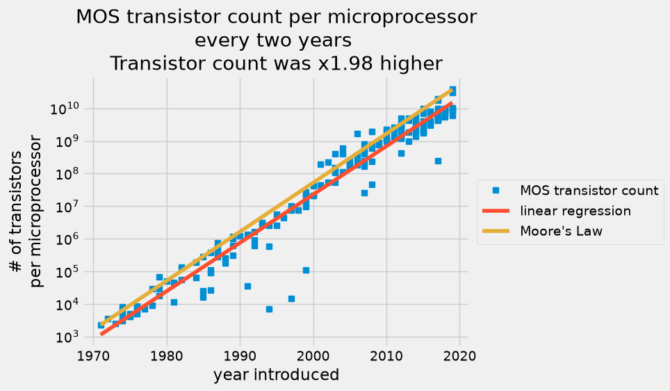
plt.ylabel("# of transistors\nper microprocessor")

A scatter plot of MOS transistor count per microprocessor every two years with a red line for the ordinary least squares prediction and an orange line for Moore’s law.

The linear regression captures the increase in the number of transistors per semiconductors each year. In 2015, semiconductor manufacturers claimed they could not keep up with Moore’s law anymore. Your analysis shows that since 1971, the average increase in transistor count was x1.98 every 2 years, but Gordon Moore predicted it would be x2 every 2 years. That is an amazing prediction.

Consider the year 2017. Compare the data to your linear regression model and Gordon Moore’s prediction. First, get the transistor counts from the year 2017. You can do this with a Boolean comparator,

year == 2017.

Then, make a prediction for 2017 with Moores_law defined above and plugging in your best fit constants into your function

\text{transistor_count} = e^{B}e^{A\cdot \text{year}}.

A great way to compare these measurements is to compare your prediction and Moore’s prediction to the average transistor count and look at the range of reported values for that year. Use the plt.plot option, alpha=0.2, to increase the transparency of the data. The more opaque the points appear, the more reported values lie on that measurement. The green $+$ is the average reported transistor count for 2017. Plot your predictions for $\pm\frac{1}{2}$ years.

transistor_count2017 = transistor_count[year == 2017]
print(
    transistor_count2017.max(), transistor_count2017.min(), transistor_count2017.mean()
)
y = np.linspace(2016.5, 2017.5)
your_model2017 = np.exp(B) * np.exp(A * y)
Moore_Model2017 = Moores_law(y)

plt.plot(
    2017 * np.ones(np.sum(year == 2017)),
    transistor_count2017,
    "ro",
    label="2017",
    alpha=0.2,
)
plt.plot(2017, transistor_count2017.mean(), "g+", markersize=20, mew=6)

plt.plot(y, your_model2017, label="Your prediction")
plt.plot(y, Moore_Model2017, label="Moores law")
plt.ylabel("# of transistors\nper microprocessor")
plt.legend()

19200000000.0 250000000.0 7050000000.0

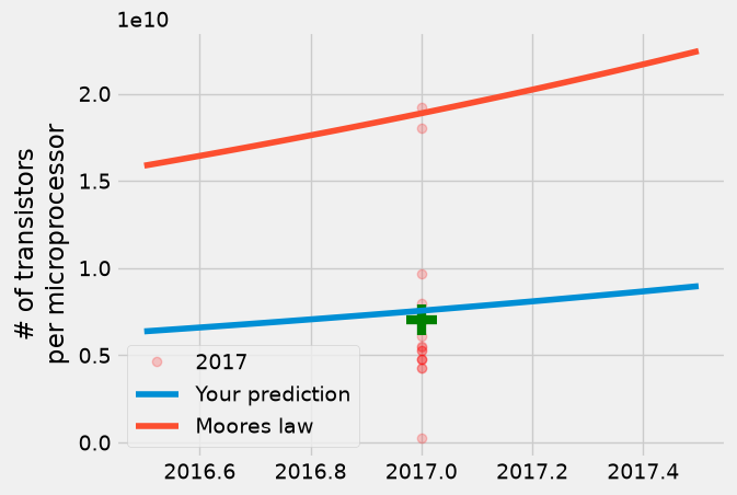
The result is that your model is close to the mean, but Gordon Moore’s prediction is closer to the maximum number of transistors per microprocessor produced in 2017. Even though semiconductor manufacturers thought that the growth would slow, once in 1975 and now again approaching 2025, manufacturers are still producing semiconductors every 2 years that nearly double the number of transistors.

The linear regression model is much better at predicting the average than extreme values because it satisfies the condition to minimize $\sum |y_i - A\cdot \text{year}[i]+B|^2$ .

The last step, is to share your findings. You created new arrays that represent a linear regression model and Gordon Moore’s prediction. You started this process by importing a csv file into a NumPy array using np.loadtxt, to save your model use two approaches

np.savez: save NumPy arrays for other Python sessions
np.savetxt: save a csv file with the original data and your predicted data

Zipping the arrays into a file¶

Using np.savez, you can save thousands of arrays and give them names. The function np.load will load the arrays back into the workspace as a dictionary. You’ll save five arrays so the next user will have the year, transistor count, predicted transistor count, Gordon Moore’s predicted count, and fitting constants. Add one more variable that other users can use to understand the model, notes.

notes = "the arrays in this file are the result of a linear regression model\n"
notes += "the arrays include\nyear: year of manufacture\n"
notes += "transistor_count: number of transistors reported by manufacturers in a given year\n"
notes += "transistor_count_predicted: linear regression model = exp({:.2f})*exp({:.2f}*year)\n".format(
    B, A
)
notes += "transistor_Moores_law: Moores law =exp({:.2f})*exp({:.2f}*year)\n".format(
    B_M, A_M
)
notes += "regression_csts: linear regression constants A and B for log(transistor_count)=A*year+B"
print(notes)

the arrays in this file are the result of a linear regression model
the arrays include
year: year of manufacture
transistor_count: number of transistors reported by manufacturers in a given year
transistor_count_predicted: linear regression model = exp(-666.33)*exp(0.34*year)
transistor_Moores_law: Moores law =exp(-675.38)*exp(0.35*year)
regression_csts: linear regression constants A and B for log(transistor_count)=A*year+B

np.savez(
    "mooreslaw_regression.npz",
    notes=notes,
    year=year,
    transistor_count=transistor_count,
    transistor_count_predicted=transistor_count_predicted,
    transistor_Moores_law=transistor_Moores_law,
    regression_csts=(A, B),
)

results = np.load("mooreslaw_regression.npz")

print(results["regression_csts"][1])

-666.3264063536233

! ls

_static
air-quality-data.csv
mooreslaw-tutorial.md
mooreslaw_regression.npz
pairing.md
save-load-arrays.md
text_preprocessing.py
transistor_data.csv
tutorial-air-quality-analysis.md
tutorial-deep-learning-on-mnist.md
tutorial-deep-reinforcement-learning-with-pong-from-pixels.md
tutorial-ma.md
tutorial-nlp-from-scratch
tutorial-nlp-from-scratch.md
tutorial-plotting-fractals
tutorial-plotting-fractals.md
tutorial-static_equilibrium.md
tutorial-style-guide.md
tutorial-svd.md
tutorial-x-ray-image-processing
tutorial-x-ray-image-processing.md
who_covid_19_sit_rep_time_series.csv
x_y-squared.csv
x_y-squared.npz

The benefit of np.savez is you can save hundreds of arrays with different shapes and types. Here, you saved 4 arrays that are double precision floating point numbers shape = (179,), one array that was text, and one array of double precision floating point numbers shape = (2,). This is the preferred method for saving NumPy arrays for use in another analysis.

Creating your own comma separated value file¶

If you want to share data and view the results in a table, then you have to create a text file. Save the data using np.savetxt. This function is more limited than np.savez. Delimited files, like csv’s, need 2D arrays.

Prepare the data for export by creating a new 2D array whose columns contain the data of interest.

Use the header option to describe the data and the columns of the file. Define another variable that contains file information as head.

head = "the columns in this file are the result of a linear regression model\n"
head += "the columns include\nyear: year of manufacture\n"
head += "transistor_count: number of transistors reported by manufacturers in a given year\n"
head += "transistor_count_predicted: linear regression model = exp({:.2f})*exp({:.2f}*year)\n".format(
    B, A
)
head += "transistor_Moores_law: Moores law =exp({:.2f})*exp({:.2f}*year)\n".format(
    B_M, A_M
)
head += "year:, transistor_count:, transistor_count_predicted:, transistor_Moores_law:"
print(head)

the columns in this file are the result of a linear regression model
the columns include
year: year of manufacture
transistor_count: number of transistors reported by manufacturers in a given year
transistor_count_predicted: linear regression model = exp(-666.33)*exp(0.34*year)
transistor_Moores_law: Moores law =exp(-675.38)*exp(0.35*year)
year:, transistor_count:, transistor_count_predicted:, transistor_Moores_law:

Build a single 2D array to export to csv. Tabular data is inherently two dimensional. You need to organize your data to fit this 2D structure. Use year, transistor_count, transistor_count_predicted, and transistor_Moores_law as the first through fourth columns, respectively. Put the calculated constants in the header since they do not fit the (179,) shape. The np.block function appends arrays together to create a new, larger array. Arrange the 1D vectors as columns using np.newaxis e.g.

>>> year.shape
(179,)
>>> year[:,np.newaxis].shape
(179,1)

output = np.block(
    [
        year[:, np.newaxis],
        transistor_count[:, np.newaxis],
        transistor_count_predicted[:, np.newaxis],
        transistor_Moores_law[:, np.newaxis],
    ]
)

Creating the mooreslaw_regression.csv with np.savetxt, use three options to create the desired file format:

X = output : use output block to write the data into the file
delimiter = ',' : use commas to separate columns in the file
header = head : use the header head defined above

np.savetxt("mooreslaw_regression.csv", X=output, delimiter=",", header=head)

! head mooreslaw_regression.csv

# the columns in this file are the result of a linear regression model
# the columns include
# year: year of manufacture
# transistor_count: number of transistors reported by manufacturers in a given year
# transistor_count_predicted: linear regression model = exp(-666.33)*exp(0.34*year)
# transistor_Moores_law: Moores law =exp(-675.38)*exp(0.35*year)
# year:, transistor_count:, transistor_count_predicted:, transistor_Moores_law:
1.971000000000000000e+03,2.250000000000000000e+03,1.130514785642591733e+03,2.249999999999916326e+03
1.972000000000000000e+03,3.500000000000000000e+03,1.590908400344571419e+03,3.181980515339620069e+03
1.973000000000000000e+03,2.500000000000000000e+03,2.238793840142739555e+03,4.500000000000097316e+03

Wrapping up¶

In conclusion, you have compared historical data for semiconductor manufacturers to Moore’s law and created a linear regression model to find the average number of transistors added to each microprocessor every two years. Gordon Moore predicted the number of transistors would double every two years from 1965 through 1975, but the average growth has maintained a consistent increase of $\times 1.98 \pm 0.01$ every two years from 1971 through 2019. In 2015, Moore revised his prediction to say Moore’s law should hold until 2025. [2]. You can share these results as a zipped NumPy array file, mooreslaw_regression.npz, or as another csv, mooreslaw_regression.csv. The amazing progress in semiconductor manufacturing has enabled new industries and computational power. This analysis should give you a small insight into how incredible this growth has been over the last half-century.

References¶

Numpy Tutorials

Applications

Deep learning on MNIST