Using the convenience classes#
The convenience classes provided by the polynomial package are:
Name |
Provides |
|---|---|
Power series |
|
Chebyshev series |
|
Legendre series |
|
Laguerre series |
|
Hermite series |
|
HermiteE series |
The series in this context are finite sums of the corresponding polynomial basis functions multiplied by coefficients. For instance, a power series looks like
and has coefficients \([1, 2, 3]\). The Chebyshev series with the same coefficients looks like
and more generally
where in this case the \(T_n\) are the Chebyshev functions of degree \(n\), but could just as easily be the basis functions of any of the other classes. The convention for all the classes is that the coefficient \(c[i]\) goes with the basis function of degree i.
All of the classes are immutable and have the same methods, and especially they implement the Python numeric operators +, -, *, //, %, divmod, **, ==, and !=. The last two can be a bit problematic due to floating point roundoff errors. We now give a quick demonstration of the various operations using NumPy version 1.7.0.
Basics#
First we need a polynomial class and a polynomial instance to play with. The classes can be imported directly from the polynomial package or from the module of the relevant type. Here we import from the package and use the conventional Polynomial class because of its familiarity:
>>> from numpy.polynomial import Polynomial as P
>>> p = P([1,2,3])
>>> p
Polynomial([1., 2., 3.], domain=[-1.,  1.], window=[-1.,  1.], symbol='x')
Note that there are three parts to the long version of the printout. The first is the coefficients, the second is the domain, and the third is the window:
>>> p.coef
array([1., 2., 3.])
>>> p.domain
array([-1.,  1.])
>>> p.window
array([-1.,  1.])
Printing a polynomial yields the polynomial expression in a more familiar format:
>>> print(p)
1.0 + 2.0·x + 3.0·x²
Note that the string representation of polynomials uses Unicode characters
by default (except on Windows) to express powers and subscripts. An ASCII-based
representation is also available (default on Windows). The polynomial string
format can be toggled at the package-level with the
set_default_printstyle function:
>>> np.polynomial.set_default_printstyle('ascii')
>>> print(p)
1.0 + 2.0 x + 3.0 x**2
or controlled for individual polynomial instances with string formatting:
>>> print(f"{p:unicode}")
1.0 + 2.0·x + 3.0·x²
We will deal with the domain and window when we get to fitting, for the moment we ignore them and run through the basic algebraic and arithmetic operations.
Addition and Subtraction:
>>> p + p
Polynomial([2., 4., 6.], domain=[-1.,  1.], window=[-1.,  1.], symbol='x')
>>> p - p
Polynomial([0.], domain=[-1.,  1.], window=[-1.,  1.], symbol='x')
Multiplication:
>>> p * p
Polynomial([ 1.,   4.,  10.,  12.,   9.], domain=[-1.,  1.], window=[-1.,  1.], symbol='x')
Powers:
>>> p**2
Polynomial([ 1.,   4., 10., 12.,  9.], domain=[-1.,  1.], window=[-1.,  1.], symbol='x')
Division:
Floor division, ‘//’, is the division operator for the polynomial classes, polynomials are treated like integers in this regard. For Python versions < 3.x the ‘/’ operator maps to ‘//’, as it does for Python, for later versions the ‘/’ will only work for division by scalars. At some point it will be deprecated:
>>> p // P([-1, 1])
Polynomial([5.,  3.], domain=[-1.,  1.], window=[-1.,  1.], symbol='x')
Remainder:
>>> p % P([-1, 1])
Polynomial([6.], domain=[-1.,  1.], window=[-1.,  1.], symbol='x')
Divmod:
>>> quo, rem = divmod(p, P([-1, 1]))
>>> quo
Polynomial([5.,  3.], domain=[-1.,  1.], window=[-1.,  1.], symbol='x')
>>> rem
Polynomial([6.], domain=[-1.,  1.], window=[-1.,  1.], symbol='x')
Evaluation:
>>> x = np.arange(5)
>>> p(x)
array([  1.,   6.,  17.,  34.,  57.])
>>> x = np.arange(6).reshape(3,2)
>>> p(x)
array([[ 1.,   6.],
       [17.,  34.],
       [57.,  86.]])
Substitution:
Substitute a polynomial for x and expand the result. Here we substitute p in itself leading to a new polynomial of degree 4 after expansion. If the polynomials are regarded as functions this is composition of functions:
>>> p(p)
Polynomial([ 6., 16., 36., 36., 27.], domain=[-1.,  1.], window=[-1.,  1.], symbol='x')
Roots:
>>> p.roots()
array([-0.33333333-0.47140452j, -0.33333333+0.47140452j])
It isn’t always convenient to explicitly use Polynomial instances, so tuples, lists, arrays, and scalars are automatically cast in the arithmetic operations:
>>> p + [1, 2, 3]
Polynomial([2., 4., 6.], domain=[-1.,  1.], window=[-1.,  1.], symbol='x')
>>> [1, 2, 3] * p
Polynomial([ 1.,  4., 10., 12.,  9.], domain=[-1.,  1.], window=[-1.,  1.], symbol='x')
>>> p / 2
Polynomial([0.5, 1. , 1.5], domain=[-1.,  1.], window=[-1.,  1.], symbol='x')
Polynomials that differ in domain, window, or class can’t be mixed in arithmetic:
>>> from numpy.polynomial import Chebyshev as T
>>> p + P([1], domain=[0,1])
Traceback (most recent call last):
  File "<stdin>", line 1, in <module>
  File "<string>", line 213, in __add__
TypeError: Domains differ
>>> p + P([1], window=[0,1])
Traceback (most recent call last):
  File "<stdin>", line 1, in <module>
  File "<string>", line 215, in __add__
TypeError: Windows differ
>>> p + T([1])
Traceback (most recent call last):
  File "<stdin>", line 1, in <module>
  File "<string>", line 211, in __add__
TypeError: Polynomial types differ
But different types can be used for substitution. In fact, this is how conversion of Polynomial classes among themselves is done for type, domain, and window casting:
>>> p(T([0, 1]))
Chebyshev([2.5, 2. , 1.5], domain=[-1.,  1.], window=[-1.,  1.], symbol='x')
Which gives the polynomial p in Chebyshev form. This works because \(T_1(x) = x\) and substituting \(x\) for \(x\) doesn’t change the original polynomial. However, all the multiplications and divisions will be done using Chebyshev series, hence the type of the result.
It is intended that all polynomial instances are immutable, therefore
augmented operations (+=, -=, etc.) and any other functionality that
would violate the immutablity of a polynomial instance are intentionally
unimplemented.
Calculus#
Polynomial instances can be integrated and differentiated.:
>>> from numpy.polynomial import Polynomial as P
>>> p = P([2, 6])
>>> p.integ()
Polynomial([0., 2., 3.], domain=[-1.,  1.], window=[-1.,  1.], symbol='x')
>>> p.integ(2)
Polynomial([0., 0., 1., 1.], domain=[-1.,  1.], window=[-1.,  1.], symbol='x')
The first example integrates p once, the second example integrates it twice. By default, the lower bound of the integration and the integration constant are 0, but both can be specified.:
>>> p.integ(lbnd=-1)
Polynomial([-1.,  2.,  3.], domain=[-1.,  1.], window=[-1.,  1.], symbol='x')
>>> p.integ(lbnd=-1, k=1)
Polynomial([0., 2., 3.], domain=[-1.,  1.], window=[-1.,  1.], symbol='x')
In the first case the lower bound of the integration is set to -1 and the integration constant is 0. In the second the constant of integration is set to 1 as well. Differentiation is simpler since the only option is the number of times the polynomial is differentiated:
>>> p = P([1, 2, 3])
>>> p.deriv(1)
Polynomial([2., 6.], domain=[-1.,  1.], window=[-1.,  1.], symbol='x')
>>> p.deriv(2)
Polynomial([6.], domain=[-1.,  1.], window=[-1.,  1.], symbol='x')
Other polynomial constructors#
Constructing polynomials by specifying coefficients is just one way of obtaining a polynomial instance, they may also be created by specifying their roots, by conversion from other polynomial types, and by least squares fits. Fitting is discussed in its own section, the other methods are demonstrated below:
>>> from numpy.polynomial import Polynomial as P
>>> from numpy.polynomial import Chebyshev as T
>>> p = P.fromroots([1, 2, 3])
>>> p
Polynomial([-6., 11., -6.,  1.], domain=[-1.,  1.], window=[-1.,  1.], symbol='x')
>>> p.convert(kind=T)
Chebyshev([-9.  , 11.75, -3.  ,  0.25], domain=[-1.,  1.], window=[-1.,  1.], symbol='x')
The convert method can also convert domain and window:
>>> p.convert(kind=T, domain=[0, 1])
Chebyshev([-2.4375 ,  2.96875, -0.5625 ,  0.03125], domain=[0.,  1.], window=[-1.,  1.], symbol='x')
>>> p.convert(kind=P, domain=[0, 1])
Polynomial([-1.875,  2.875, -1.125,  0.125], domain=[0.,  1.], window=[-1.,  1.], symbol='x')
In numpy versions >= 1.7.0 the basis and cast class methods are also available. The cast method works like the convert method while the basis method returns the basis polynomial of given degree:
>>> P.basis(3)
Polynomial([0., 0., 0., 1.], domain=[-1.,  1.], window=[-1.,  1.], symbol='x')
>>> T.cast(p)
Chebyshev([-9.  , 11.75, -3. ,  0.25], domain=[-1.,  1.], window=[-1.,  1.], symbol='x')
Conversions between types can be useful, but it is not recommended for routine use. The loss of numerical precision in passing from a Chebyshev series of degree 50 to a Polynomial series of the same degree can make the results of numerical evaluation essentially random.
Fitting#
Fitting is the reason that the domain and window attributes are part of the convenience classes. To illustrate the problem, the values of the Chebyshev polynomials up to degree 5 are plotted below.
>>> import matplotlib.pyplot as plt
>>> from numpy.polynomial import Chebyshev as T
>>> x = np.linspace(-1, 1, 100)
>>> for i in range(6):
...     ax = plt.plot(x, T.basis(i)(x), lw=2, label=f"$T_{i}$")
...
>>> plt.legend(loc="upper left")
>>> plt.show()
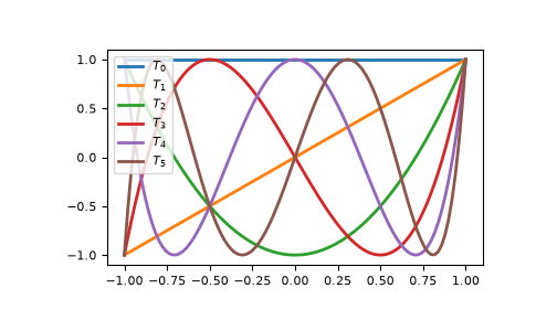
In the range -1 <= x <= 1 they are nice, equiripple functions lying between +/- 1. The same plots over the range -2 <= x <= 2 look very different:
>>> import matplotlib.pyplot as plt
>>> from numpy.polynomial import Chebyshev as T
>>> x = np.linspace(-2, 2, 100)
>>> for i in range(6):
...     ax = plt.plot(x, T.basis(i)(x), lw=2, label=f"$T_{i}$")
...
>>> plt.legend(loc="lower right")
>>> plt.show()
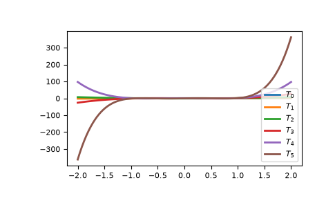
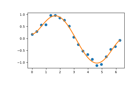
As can be seen, the “good” parts have shrunk to insignificance. In using Chebyshev polynomials for fitting we want to use the region where x is between -1 and 1 and that is what the window specifies. However, it is unlikely that the data to be fit has all its data points in that interval, so we use domain to specify the interval where the data points lie. When the fit is done, the domain is first mapped to the window by a linear transformation and the usual least squares fit is done using the mapped data points. The window and domain of the fit are part of the returned series and are automatically used when computing values, derivatives, and such. If they aren’t specified in the call the fitting routine will use the default window and the smallest domain that holds all the data points. This is illustrated below for a fit to a noisy sine curve.
>>> import numpy as np
>>> import matplotlib.pyplot as plt
>>> from numpy.polynomial import Chebyshev as T
>>> np.random.seed(11)
>>> x = np.linspace(0, 2*np.pi, 20)
>>> y = np.sin(x) + np.random.normal(scale=.1, size=x.shape)
>>> p = T.fit(x, y, 5)
>>> plt.plot(x, y, 'o')
>>> xx, yy = p.linspace()
>>> plt.plot(xx, yy, lw=2)
>>> p.domain
array([0.        ,  6.28318531])
>>> p.window
array([-1.,  1.])
>>> plt.show()