numpy.fft.ifftn#

fft.ifftn(a, s=None, axes=None, norm=None, out=None)[source]#

Compute the N-dimensional inverse discrete Fourier Transform.

This function computes the inverse of the N-dimensional discrete Fourier Transform over any number of axes in an M-dimensional array by means of the Fast Fourier Transform (FFT). In other words, ifftn(fftn(a)) == a to within numerical accuracy. For a description of the definitions and conventions used, see numpy.fft.

The input, analogously to ifft, should be ordered in the same way as is returned by fftn, i.e. it should have the term for zero frequency in all axes in the low-order corner, the positive frequency terms in the first half of all axes, the term for the Nyquist frequency in the middle of all axes and the negative frequency terms in the second half of all axes, in order of decreasingly negative frequency.

Parameters:

aarray_like

Input array, can be complex.

ssequence of ints, optional

Shape (length of each transformed axis) of the output (s[0] refers to axis 0, s[1] to axis 1, etc.). This corresponds to n for ifft(x, n). Along any axis, if the given shape is smaller than that of the input, the input is cropped. If it is larger, the input is padded with zeros.

Changed in version 2.0: If it is -1, the whole input is used (no padding/trimming).

If s is not given, the shape of the input along the axes specified by axes is used. See notes for issue on ifft zero padding.

Deprecated since version 2.0: If s is not None, axes must not be None either.

Deprecated since version 2.0: s must contain only int s, not None values. None values currently mean that the default value for n is used in the corresponding 1-D transform, but this behaviour is deprecated.

axessequence of ints, optional

Axes over which to compute the IFFT. If not given, the last len(s) axes are used, or all axes if s is also not specified. Repeated indices in axes means that the inverse transform over that axis is performed multiple times.

Deprecated since version 2.0: If s is specified, the corresponding axes to be transformed must be explicitly specified too.

norm{“backward”, “ortho”, “forward”}, optional

New in version 1.10.0.

Normalization mode (see numpy.fft). Default is “backward”. Indicates which direction of the forward/backward pair of transforms is scaled and with what normalization factor.

New in version 1.20.0: The “backward”, “forward” values were added.

outcomplex ndarray, optional

If provided, the result will be placed in this array. It should be of the appropriate shape and dtype for all axes (and hence is incompatible with passing in all but the trivial s).

New in version 2.0.0.

Returns:

outcomplex ndarray: The truncated or zero-padded input, transformed along the axes indicated by axes, or by a combination of s or a, as explained in the parameters section above.

Raises:

ValueError: If s and axes have different length.
IndexError: If an element of axes is larger than than the number of axes of a.

See also

numpy.fft: Overall view of discrete Fourier transforms, with definitions and conventions used.
fftn: The forward n-dimensional FFT, of which ifftn is the inverse.
ifft: The one-dimensional inverse FFT.
ifft2: The two-dimensional inverse FFT.
ifftshift: Undoes fftshift, shifts zero-frequency terms to beginning of array.

Notes

See numpy.fft for definitions and conventions used.

Zero-padding, analogously with ifft, is performed by appending zeros to the input along the specified dimension. Although this is the common approach, it might lead to surprising results. If another form of zero padding is desired, it must be performed before ifftn is called.

Examples

>>> import numpy as np
>>> a = np.eye(4)
>>> np.fft.ifftn(np.fft.fftn(a, axes=(0,)), axes=(1,))
array([[1.+0.j,  0.+0.j,  0.+0.j,  0.+0.j], # may vary
       [0.+0.j,  1.+0.j,  0.+0.j,  0.+0.j],
       [0.+0.j,  0.+0.j,  1.+0.j,  0.+0.j],
       [0.+0.j,  0.+0.j,  0.+0.j,  1.+0.j]])

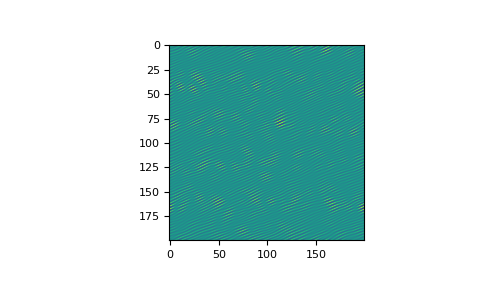
Create and plot an image with band-limited frequency content:

>>> import matplotlib.pyplot as plt
>>> n = np.zeros((200,200), dtype=complex)
>>> n[60:80, 20:40] = np.exp(1j*np.random.uniform(0, 2*np.pi, (20, 20)))
>>> im = np.fft.ifftn(n).real
>>> plt.imshow(im)
<matplotlib.image.AxesImage object at 0x...>
>>> plt.show()