numpy.linalg.lstsq#

linalg.lstsq(a, b, rcond=None)[source]#

Return the least-squares solution to a linear matrix equation.

Computes the vector x that approximately solves the equation a @ x = b. The equation may be under-, well-, or over-determined (i.e., the number of linearly independent rows of a can be less than, equal to, or greater than its number of linearly independent columns). If a is square and of full rank, then x (but for round-off error) is the “exact” solution of the equation. Else, x minimizes the Euclidean 2-norm \(||b - ax||\). If there are multiple minimizing solutions, the one with the smallest 2-norm \(||x||\) is returned.

Parameters:

a(M, N) array_like: “Coefficient” matrix.
b{(M,), (M, K)} array_like: Ordinate or “dependent variable” values. If b is two-dimensional, the least-squares solution is calculated for each of the K columns of b.
rcondfloat, optional: Cut-off ratio for small singular values of a. For the purposes of rank determination, singular values are treated as zero if they are smaller than rcond times the largest singular value of a. The default uses the machine precision times max(M, N). Passing -1 will use machine precision.

Changed in version 2.0: Previously, the default was -1, but a warning was given that this would change.

Returns:

x{(N,), (N, K)} ndarray: Least-squares solution. If b is two-dimensional, the solutions are in the K columns of x.
residuals{(1,), (K,), (0,)} ndarray: Sums of squared residuals: Squared Euclidean 2-norm for each column in b - a @ x. If the rank of a is < N or M <= N, this is an empty array. If b is 1-dimensional, this is a (1,) shape array. Otherwise the shape is (K,).
rankint: Rank of matrix a.
s(min(M, N),) ndarray: Singular values of a.

Raises:

LinAlgError: If computation does not converge.

See also

scipy.linalg.lstsq: Similar function in SciPy.

Notes

If b is a matrix, then all array results are returned as matrices.

Examples

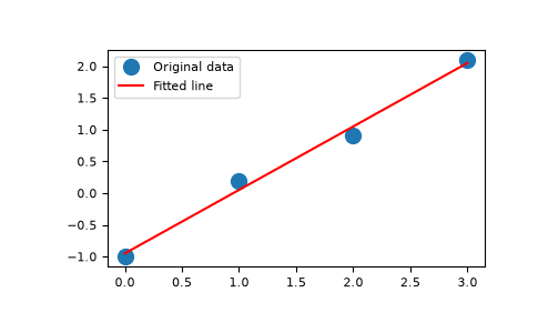
Fit a line, y = mx + c, through some noisy data-points:

>>> import numpy as np
>>> x = np.array([0, 1, 2, 3])
>>> y = np.array([-1, 0.2, 0.9, 2.1])

By examining the coefficients, we see that the line should have a gradient of roughly 1 and cut the y-axis at, more or less, -1.

We can rewrite the line equation as y = Ap, where A = [[x 1]] and p = [[m], [c]]. Now use lstsq to solve for p:

>>> A = np.vstack([x, np.ones(len(x))]).T
>>> A
array([[ 0.,  1.],
       [ 1.,  1.],
       [ 2.,  1.],
       [ 3.,  1.]])

>>> m, c = np.linalg.lstsq(A, y)[0]
>>> m, c
(1.0 -0.95) # may vary

Plot the data along with the fitted line:

>>> import matplotlib.pyplot as plt
>>> _ = plt.plot(x, y, 'o', label='Original data', markersize=10)
>>> _ = plt.plot(x, m*x + c, 'r', label='Fitted line')
>>> _ = plt.legend()
>>> plt.show()