numpy.random.Generator.chisquare

method

random.Generator.chisquare(df, size=None)

Draw samples from a chi-square distribution.

When df independent random variables, each with standard normal distributions (mean 0, variance 1), are squared and summed, the resulting distribution is chi-square (see Notes). This distribution is often used in hypothesis testing.

Parameters:

dffloat or array_like of floats

Number of degrees of freedom, must be > 0.

sizeint or tuple of ints, optional

Output shape. If the given shape is, e.g., (m, n, k), then m * n * k samples are drawn. If size is None (default), a single value is returned if df is a scalar. Otherwise, np.array(df).size samples are drawn.

Returns:

outndarray or scalar

Drawn samples from the parameterized chi-square distribution.

Raises:

ValueError

When df <= 0 or when an inappropriate size (e.g. size=-1) is given.

Notes

The variable obtained by summing the squares of df independent, standard normally distributed random variables:

\[Q = \sum_{i=0}^{\mathtt{df}} X^2_i\]

is chi-square distributed, denoted

\[Q \sim \chi^2_k.\]

The probability density function of the chi-squared distribution is

\[p(x) = \frac{(1/2)^{k/2}}{\Gamma(k/2)} x^{k/2 - 1} e^{-x/2},\]

where \(\Gamma\) is the gamma function,

\[\Gamma(x) = \int_0^{-\infty} t^{x - 1} e^{-t} dt.\]

References

[1]

NIST “Engineering Statistics Handbook” https://www.itl.nist.gov/div898/handbook/eda/section3/eda3666.htm

Examples

>>> rng = np.random.default_rng()
>>> rng.chisquare(2,4)
array([ 1.89920014,  9.00867716,  3.13710533,  5.62318272]) # random

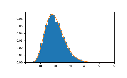
The distribution of a chi-square random variable with 20 degrees of freedom looks as follows:

>>> import matplotlib.pyplot as plt
>>> import scipy.stats as stats
>>> s = rng.chisquare(20, 10000)
>>> count, bins, _ = plt.hist(s, 30, density=True)
>>> x = np.linspace(0, 60, 1000)
>>> plt.plot(x, stats.chi2.pdf(x, df=20))
>>> plt.xlim([0, 60])
>>> plt.show()