numpy.random.Generator.normal

method

random.Generator.normal(loc=0.0, scale=1.0, size=None)

Draw random samples from a normal (Gaussian) distribution.

The probability density function of the normal distribution, first derived by De Moivre and 200 years later by both Gauss and Laplace independently [2], is often called the bell curve because of its characteristic shape (see the example below).

The normal distributions occurs often in nature. For example, it describes the commonly occurring distribution of samples influenced by a large number of tiny, random disturbances, each with its own unique distribution [2].

Parameters:

locfloat or array_like of floats

Mean (“centre”) of the distribution.

scalefloat or array_like of floats

Standard deviation (spread or “width”) of the distribution. Must be non-negative.

sizeint or tuple of ints, optional

Output shape. If the given shape is, e.g., (m, n, k), then m * n * k samples are drawn. If size is None (default), a single value is returned if loc and scale are both scalars. Otherwise, np.broadcast(loc, scale).size samples are drawn.

Returns:

outndarray or scalar

Drawn samples from the parameterized normal distribution.

See also

scipy.stats.norm

probability density function, distribution or cumulative density function, etc.

Notes

The probability density for the Gaussian distribution is

\[p(x) = \frac{1}{\sqrt{ 2 \pi \sigma^2 }} e^{ - \frac{ (x - \mu)^2 } {2 \sigma^2} },\]

where \(\mu\) is the mean and \(\sigma\) the standard deviation. The square of the standard deviation, \(\sigma^2\), is called the variance.

The function has its peak at the mean, and its “spread” increases with the standard deviation (the function reaches 0.607 times its maximum at \(x + \sigma\) and \(x - \sigma\) [2]). This implies that normal is more likely to return samples lying close to the mean, rather than those far away.

References

[1]

Wikipedia, “Normal distribution”, https://en.wikipedia.org/wiki/Normal_distribution

[2] (1,2,3)

P. R. Peebles Jr., “Central Limit Theorem” in “Probability, Random Variables and Random Signal Principles”, 4th ed., 2001, pp. 51, 51, 125.

Examples

Try it in your browser!

Draw samples from the distribution:

>>> mu, sigma = 0, 0.1 # mean and standard deviation
>>> rng = np.random.default_rng()
>>> s = rng.normal(mu, sigma, 1000)

Verify the mean and the standard deviation:

>>> abs(mu - np.mean(s))
0.0  # may vary

>>> abs(sigma - np.std(s, ddof=1))
0.0  # may vary

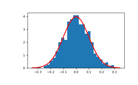
Display the histogram of the samples, along with the probability density function:

>>> import matplotlib.pyplot as plt
>>> count, bins, _ = plt.hist(s, 30, density=True)
>>> plt.plot(bins, 1/(sigma * np.sqrt(2 * np.pi)) *
...                np.exp( - (bins - mu)**2 / (2 * sigma**2) ),
...          linewidth=2, color='r')
>>> plt.show()

Two-by-four array of samples from the normal distribution with mean 3 and standard deviation 2.5:

>>> rng = np.random.default_rng()
>>> rng.normal(3, 2.5, size=(2, 4))
array([[-4.49401501,  4.00950034, -1.81814867,  7.29718677],   # random
       [ 0.39924804,  4.68456316,  4.99394529,  4.84057254]])  # random

Go BackOpen In Tab