
X-ray image processing#
This tutorial demonstrates how to read and process X-ray images with NumPy, imageio, Matplotlib and SciPy. You will learn how to load medical images, focus on certain parts, and visually compare them using the Gaussian, Laplacian-Gaussian, Sobel, and Canny filters for edge detection.
X-ray image analysis can be part of your data analysis and machine learning workflow when, for example, you’re building an algorithm that helps detect pneumonia as part of a Kaggle competition. In the healthcare industry, medical image processing and analysis is particularly important when images are estimated to account for at least 90% of all medical data.
You’ll be working with radiology images from the
ChestX-ray8
dataset provided by the National Institutes of Health (NIH).
ChestX-ray8 contains over 100,000 de-identified X-ray images in the PNG format
from more than 30,000 patients. You can find ChestX-ray8’s files on NIH’s public
Box repository in the /images
folder. (For more details, refer to the research
paper
published at CVPR (a computer vision conference) in 2017.)
For your convenience, a small number of PNG images have been saved to this
tutorial’s repository under tutorial-x-ray-image-processing/, since
ChestX-ray8 contains gigabytes of data and you may find it challenging to
download it in batches.

Prerequisites#
The reader should have some knowledge of Python, NumPy arrays, and Matplotlib. To refresh the memory, you can take the Python and Matplotlib PyPlot tutorials, and the NumPy quickstart.
The following packages are used in this tutorial:
imageio for reading and writing image data. The healthcare industry usually works with the DICOM format for medical imaging and imageio should be well-suited for reading that format. For simplicity, in this tutorial you’ll be working with PNG files.
Matplotlib for data visualization.
This tutorial can be run locally in an isolated environment, such as Virtualenv or conda. You can use Jupyter Notebook or JupyterLab to run each notebook cell.
Table of contents#
Examine an X-ray with
imageioCombine images into a multi-dimensional array to demonstrate progression
Edge detection using the Laplacian-Gaussian, Gaussian gradient, Sobel, and Canny filters
Apply masks to X-rays with
np.where()Compare the results
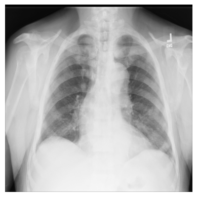
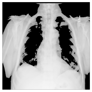
Examine an X-ray with imageio#
Let’s begin with a simple example using just one X-ray image from the ChestX-ray8 dataset.
The file — 00000011_001.png — has been downloaded for you and saved in the
/tutorial-x-ray-image-processing folder.
1. Load the image with imageio:
import os
import imageio

DIR = "tutorial-x-ray-image-processing"

xray_image = imageio.v3.imread(os.path.join(DIR, "00000011_001.png"))
2. Check that its shape is 1024x1024 pixels and that the array is made up of 8-bit integers:
print(xray_image.shape)
print(xray_image.dtype)
(1024, 1024)
uint8
3. Import matplotlib and display the image in a grayscale colormap:
import matplotlib.pyplot as plt

plt.imshow(xray_image, cmap="gray")
plt.axis("off")
plt.show()
Combine images into a multidimensional array to demonstrate progression#
In the next example, instead of 1 image you’ll use 9 X-ray 1024x1024-pixel
images from the ChestX-ray8 dataset that have been downloaded and extracted
from one of the dataset files. They are numbered from ...000.png to
...008.png and let’s assume they belong to the same patient.
1. Import NumPy, read in each of the X-rays, and create a three-dimensional array where the first dimension corresponds to image number:
import numpy as np
num_imgs = 9

combined_xray_images_1 = np.array(
    [imageio.v3.imread(os.path.join(DIR, f"00000011_00{i}.png")) for i in range(num_imgs)]
)
2. Check the shape of the new X-ray image array containing 9 stacked images:
combined_xray_images_1.shape
(9, 1024, 1024)
Note that the shape in the first dimension matches num_imgs, so the
combined_xray_images_1 array can be interpreted as a stack of 2D images.
3. You can now display the “health progress” by plotting each of frames next to each other using Matplotlib:
fig, axes = plt.subplots(nrows=1, ncols=num_imgs, figsize=(30, 30))

for img, ax in zip(combined_xray_images_1, axes):
    ax.imshow(img, cmap='gray')
    ax.axis('off')
4. In addition, it can be helpful to show the progress as an animation.
Let’s create a GIF file with imageio.mimwrite() and display the result in the
notebook:
GIF_PATH = os.path.join(DIR, "xray_image.gif")
imageio.mimwrite(GIF_PATH, combined_xray_images_1, format= ".gif", duration=1000)
Which gives us:
Edge detection using the Laplacian-Gaussian, Gaussian gradient, Sobel, and Canny filters#
When processing biomedical data, it can be useful to emphasize the 2D “edges” to focus on particular features in an image. To do that, using image gradients can be particularly helpful when detecting the change of color pixel intensity.
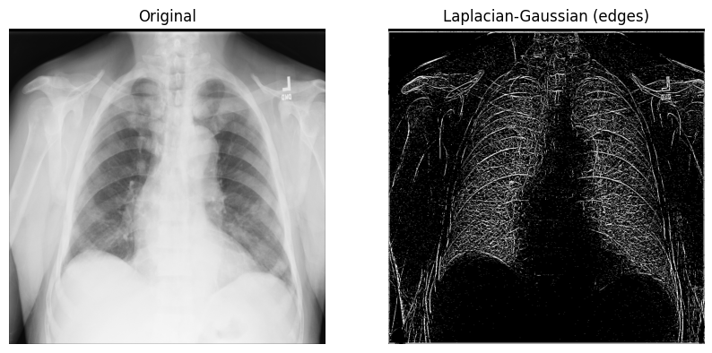
The Laplace filter with Gaussian second derivatives#
Let’s start with an n-dimensional Laplace filter (“Laplacian-Gaussian”) that uses Gaussian second derivatives. This Laplacian method focuses on pixels with rapid intensity change in values and is combined with Gaussian smoothing to remove noise. Let’s examine how it can be useful in analyzing 2D X-ray images.
The implementation of the Laplacian-Gaussian filter is relatively straightforward: 1) import the
ndimagemodule from SciPy; and 2) callscipy.ndimage.gaussian_laplace()with a sigma (scalar) parameter, which affects the standard deviations of the Gaussian filter (you’ll use1in the example below):
from scipy import ndimage

xray_image_laplace_gaussian = ndimage.gaussian_laplace(xray_image, sigma=1)
Display the original X-ray and the one with the Laplacian-Gaussian filter:
fig, axes = plt.subplots(nrows=1, ncols=2, figsize=(10, 10))

axes[0].set_title("Original")
axes[0].imshow(xray_image, cmap="gray")
axes[1].set_title("Laplacian-Gaussian (edges)")
axes[1].imshow(xray_image_laplace_gaussian, cmap="gray")
for i in axes:
    i.axis("off")
plt.show()
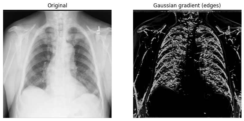
The Gaussian gradient magnitude method#
Another method for edge detection that can be useful is the Gaussian (gradient) filter. It computes the multidimensional gradient magnitude with Gaussian derivatives and helps by remove high-frequency image components.
1. Call scipy.ndimage.gaussian_gradient_magnitude()
with a sigma (scalar) parameter (for standard deviations; you’ll use 2 in the
example below):
x_ray_image_gaussian_gradient = ndimage.gaussian_gradient_magnitude(xray_image, sigma=2)
2. Display the original X-ray and the one with the Gaussian gradient filter:
fig, axes = plt.subplots(nrows=1, ncols=2, figsize=(10, 10))

axes[0].set_title("Original")
axes[0].imshow(xray_image, cmap="gray")
axes[1].set_title("Gaussian gradient (edges)")
axes[1].imshow(x_ray_image_gaussian_gradient, cmap="gray")
for i in axes:
    i.axis("off")
plt.show()
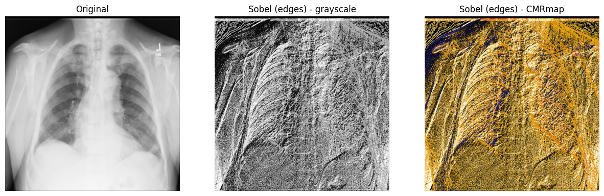
The Sobel-Feldman operator (the Sobel filter)#
To find regions of high spatial frequency (the edges or the edge maps) along the horizontal and vertical axes of a 2D X-ray image, you can use the Sobel-Feldman operator (Sobel filter) technique. The Sobel filter applies two 3x3 kernel matrices — one for each axis — onto the X-ray through a convolution. Then, these two points (gradients) are combined using the Pythagorean theorem to produce a gradient magnitude.
1. Use the Sobel filters — (scipy.ndimage.sobel())
— on x- and y-axes of the X-ray. Then, calculate the distance between x and
y (with the Sobel filters applied to them) using the
Pythagorean theorem and
NumPy’s np.hypot()
to obtain the magnitude. Finally, normalize the rescaled image for the pixel
values to be between 0 and 255.
Image normalization
follows the output_channel = 255.0 * (input_channel - min_value) / (max_value - min_value)
formula. Because you’re
using a grayscale image, you need to normalize just one channel.
x_sobel = ndimage.sobel(xray_image, axis=0)
y_sobel = ndimage.sobel(xray_image, axis=1)

xray_image_sobel = np.hypot(x_sobel, y_sobel)

xray_image_sobel *= 255.0 / np.max(xray_image_sobel)
2. Change the new image array data type to the 32-bit floating-point format
from float16 to make it compatible
with Matplotlib:
print("The data type - before: ", xray_image_sobel.dtype)

xray_image_sobel = xray_image_sobel.astype("float32")

print("The data type - after: ", xray_image_sobel.dtype)
The data type - before:  float16
The data type - after:  float32
3. Display the original X-ray and the one with the Sobel “edge” filter
applied. Note that both the grayscale and CMRmap colormaps are used to help
emphasize the edges:
fig, axes = plt.subplots(nrows=1, ncols=3, figsize=(15, 15))

axes[0].set_title("Original")
axes[0].imshow(xray_image, cmap="gray")
axes[1].set_title("Sobel (edges) - grayscale")
axes[1].imshow(xray_image_sobel, cmap="gray")
axes[2].set_title("Sobel (edges) - CMRmap")
axes[2].imshow(xray_image_sobel, cmap="CMRmap")
for i in axes:
    i.axis("off")
plt.show()
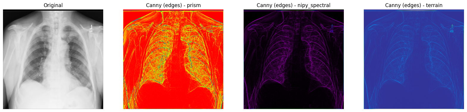
The Canny filter#
You can also consider using another well-known filter for edge detection called the Canny filter.
First, you apply a Gaussian filter to remove the noise in an image. In this example, you’re using using the Fourier filter which smoothens the X-ray through a convolution process. Next, you apply the Prewitt filter on each of the 2 axes of the image to help detect some of the edges — this will result in 2 gradient values. Similar to the Sobel filter, the Prewitt operator also applies two 3x3 kernel matrices — one for each axis — onto the X-ray through a convolution. In the end, you compute the magnitude between the two gradients using the Pythagorean theorem and normalize the images, as before.
1. Use SciPy’s Fourier filters — scipy.ndimage.fourier_gaussian()
— with a small sigma value to remove some of the noise from the X-ray. Then,
calculate two gradients using scipy.ndimage.prewitt().
Next, measure the distance between the gradients using NumPy’s np.hypot().
Finally, normalize
the rescaled image, as before.
fourier_gaussian = ndimage.fourier_gaussian(xray_image, sigma=0.05)

x_prewitt = ndimage.prewitt(fourier_gaussian, axis=0)
y_prewitt = ndimage.prewitt(fourier_gaussian, axis=1)

xray_image_canny = np.hypot(x_prewitt, y_prewitt)

xray_image_canny *= 255.0 / np.max(xray_image_canny)

print("The data type - ", xray_image_canny.dtype)
The data type - float64
2. Plot the original X-ray image and the ones with the edges detected with
the help of the Canny filter technique. The edges can be emphasized using the
prism, nipy_spectral, and terrain Matplotlib colormaps.
fig, axes = plt.subplots(nrows=1, ncols=4, figsize=(20, 15))

axes[0].set_title("Original")
axes[0].imshow(xray_image, cmap="gray")
axes[1].set_title("Canny (edges) - prism")
axes[1].imshow(xray_image_canny, cmap="prism")
axes[2].set_title("Canny (edges) - nipy_spectral")
axes[2].imshow(xray_image_canny, cmap="nipy_spectral")
axes[3].set_title("Canny (edges) - terrain")
axes[3].imshow(xray_image_canny, cmap="terrain")
for i in axes:
    i.axis("off")
plt.show()
Apply masks to X-rays with np.where()#
To screen out only certain pixels in X-ray images to help detect particular
features, you can apply masks with NumPy’s
np.where(condition: array_like (bool), x: array_like, y: ndarray)
that returns x when True and y when False.
Identifying regions of interest — certain sets of pixels in an image — can be useful and masks serve as boolean arrays of the same shape as the original image.
1. Retrieve some basics statistics about the pixel values in the original X-ray image you’ve been working with:
print("The data type of the X-ray image is: ", xray_image.dtype)
print("The minimum pixel value is: ", np.min(xray_image))
print("The maximum pixel value is: ", np.max(xray_image))
print("The average pixel value is: ", np.mean(xray_image))
print("The median pixel value is: ", np.median(xray_image))
The data type of the X-ray image is:  uint8
The minimum pixel value is:  0
The maximum pixel value is:  255
The average pixel value is:  172.52233219146729
The median pixel value is:  195.0
2. The array data type is uint8 and the minimum/maximum value results
suggest that all 256 colors (from 0 to 255) are used in the X-ray. Let’s
visualize the pixel intensity distribution of the original raw X-ray image
with ndimage.histogram() and Matplotlib:
pixel_intensity_distribution = ndimage.histogram(
    xray_image, min=np.min(xray_image), max=np.max(xray_image), bins=256
)

plt.plot(pixel_intensity_distribution)
plt.title("Pixel intensity distribution")
plt.show()
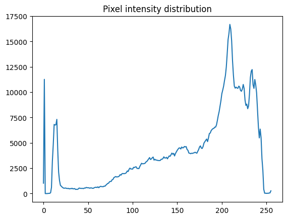
As the pixel intensity distribution suggests, there are many low (between around 0 and 20) and very high (between around 200 and 240) pixel values.
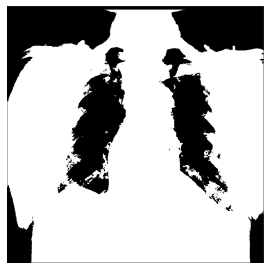
3. You can create different conditional masks with NumPy’s np.where() —
for example, let’s have only those values of the image with the pixels exceeding
a certain threshold:
# The threshold is "greater than 150"
# Return the original image if true, `0` otherwise
xray_image_mask_noisy = np.where(xray_image > 150, xray_image, 0)

plt.imshow(xray_image_mask_noisy, cmap="gray")
plt.axis("off")
plt.show()
# The threshold is "greater than 150"
# Return `1` if true, `0` otherwise
xray_image_mask_less_noisy = np.where(xray_image > 150, 1, 0)

plt.imshow(xray_image_mask_less_noisy, cmap="gray")
plt.axis("off")
plt.show()
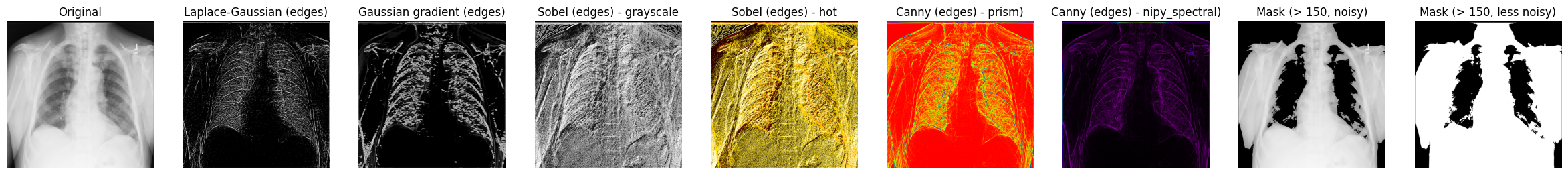
Compare the results#
Let’s display some of the results of processed X-ray images you’ve worked with so far:
fig, axes = plt.subplots(nrows=1, ncols=9, figsize=(30, 30))

axes[0].set_title("Original")
axes[0].imshow(xray_image, cmap="gray")
axes[1].set_title("Laplace-Gaussian (edges)")
axes[1].imshow(xray_image_laplace_gaussian, cmap="gray")
axes[2].set_title("Gaussian gradient (edges)")
axes[2].imshow(x_ray_image_gaussian_gradient, cmap="gray")
axes[3].set_title("Sobel (edges) - grayscale")
axes[3].imshow(xray_image_sobel, cmap="gray")
axes[4].set_title("Sobel (edges) - hot")
axes[4].imshow(xray_image_sobel, cmap="hot")
axes[5].set_title("Canny (edges) - prism)")
axes[5].imshow(xray_image_canny, cmap="prism")
axes[6].set_title("Canny (edges) - nipy_spectral)")
axes[6].imshow(xray_image_canny, cmap="nipy_spectral")
axes[7].set_title("Mask (> 150, noisy)")
axes[7].imshow(xray_image_mask_noisy, cmap="gray")
axes[8].set_title("Mask (> 150, less noisy)")
axes[8].imshow(xray_image_mask_less_noisy, cmap="gray")
for i in axes:
    i.axis("off")
plt.show()
Next steps#
If you want to use your own samples, you can use this image or search for various other ones on the Openi database. Openi contains many biomedical images and it can be especially helpful if you have low bandwidth and/or are restricted by the amount of data you can download.
To learn more about image processing in the context of biomedical image data or simply edge detection, you may find the following material useful:
DICOM processing and segmentation in Python with Scikit-Image and pydicom (Radiology Data Quest)
Image manipulation and processing using Numpy and Scipy (Scipy Lecture Notes)
Intensity values (presentation, DataCamp)
Object detection with Raspberry Pi and Python (Maker Portal)
X-ray data preparation and segmentation with deep learning (a Kaggle-hosted Jupyter notebook)
Image filtering (lecture slides, CS6670: Computer Vision, Cornell University)
Edge detection in Python and NumPy (Towards Data Science)
Edge detection with Scikit-Image (Data Carpentry)
Image gradients and gradient filtering (lecture slides, 16-385 Computer Vision, Carnegie Mellon University)