numpy.random.standard_cauchy

random.standard_cauchy(size=None)

Draw samples from a standard Cauchy distribution with mode = 0.

Also known as the Lorentz distribution.

Note

New code should use the standard_cauchy method of a Generator instance instead; please see the Quick Start.

Parameters:

sizeint or tuple of ints, optional

Output shape. If the given shape is, e.g., (m, n, k), then m * n * k samples are drawn. Default is None, in which case a single value is returned.

Returns:

samplesndarray or scalar

The drawn samples.

See also

random.Generator.standard_cauchy

which should be used for new code.

Notes

The probability density function for the full Cauchy distribution is

\[P(x; x_0, \gamma) = \frac{1}{\pi \gamma \bigl[ 1+ (\frac{x-x_0}{\gamma})^2 \bigr] }\]

and the Standard Cauchy distribution just sets \(x_0=0\) and \(\gamma=1\)

The Cauchy distribution arises in the solution to the driven harmonic oscillator problem, and also describes spectral line broadening. It also describes the distribution of values at which a line tilted at a random angle will cut the x axis.

When studying hypothesis tests that assume normality, seeing how the tests perform on data from a Cauchy distribution is a good indicator of their sensitivity to a heavy-tailed distribution, since the Cauchy looks very much like a Gaussian distribution, but with heavier tails.

References

[1]

NIST/SEMATECH e-Handbook of Statistical Methods, “Cauchy Distribution”, https://www.itl.nist.gov/div898/handbook/eda/section3/eda3663.htm

[2]

Weisstein, Eric W. “Cauchy Distribution.” From MathWorld–A Wolfram Web Resource. http://mathworld.wolfram.com/CauchyDistribution.html

[3]

Wikipedia, “Cauchy distribution” https://en.wikipedia.org/wiki/Cauchy_distribution

Examples

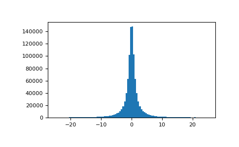
Draw samples and plot the distribution:

>>> import matplotlib.pyplot as plt
>>> s = np.random.standard_cauchy(1000000)
>>> s = s[(s>-25) & (s<25)]  # truncate distribution so it plots well
>>> plt.hist(s, bins=100)
>>> plt.show()