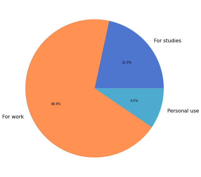
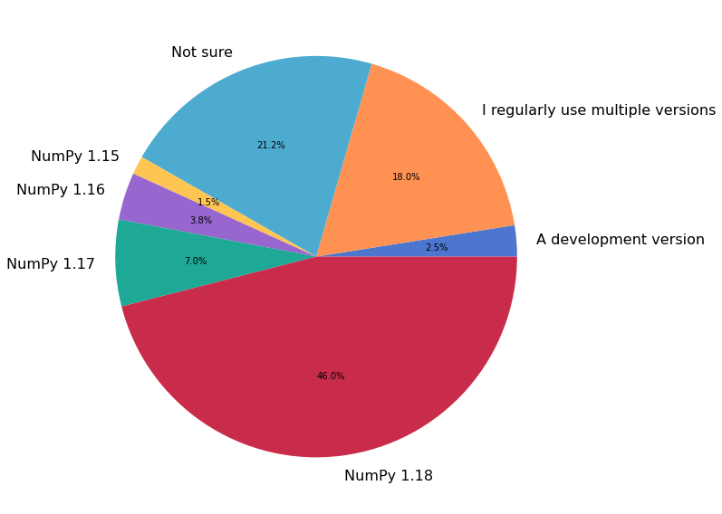
Community

A summary of the demographic information of the NumPy survey respondents.

fname = "data/2020/numpy_survey_results.tsv"
column_names = [
    'age', 'gender', 'lang', 'lang_other', 'country', 'degree', 'degree_other',
    'field_of_study', 'field_other', 'role', 'role_other', 'version', 
    'primary_use', 'programming_exp', 'numpy_exp', 'use_freq', 'components',
    'use_c_ext', 'prog_lang', 'prog_lang_other',
]
demographics_dtype = np.dtype({
    "names": column_names,
    "formats": ['<U600'] * len(column_names),
})

data = np.loadtxt(
    fname, delimiter='\t', skiprows=3, dtype=demographics_dtype, 
    usecols=range(11, 31), comments=None
)

glue('num_respondents', data.shape[0], display=False)

Demographics

Age

Of the 1236 survey respondents, 1089 (88%) shared their age.

age = data['age']
# Preprocessing
ignore_chars = ('', '> 40')
for value in ignore_chars:
    age = age[age != value]
age = age.astype(int)
# Distribution
bwidth = 10
bedges = np.arange(0, age.max() + bwidth, bwidth)
h, _ = np.histogram(age, bins=bedges)
h = 100 * h / h.sum()

fig, ax = plt.subplots(figsize=(12, 8))
x = np.arange(len(h))
ax.bar(x, h)
labels = [f"{low}-{high - 1}" for low, high in zip(bedges[:-1], bedges[1:])]
ax.set_xticks(x)
ax.set_xticklabels(labels)
fig.autofmt_xdate();
ax.set_title("Age Distribution of Survey Respondents");
ax.set_xlabel("Age (yrs)");
ax.set_ylabel("Percentage of Respondents");

glue('num_age_respondents', gluval(age.shape[0], data.shape[0]), display=False)
../../_images/demographics_5_1.png

Gender

Of the 1236 survey respondents, 1100 (89%) shared their gender.

# Ignore empty fields and "prefer not to answer"
drop = np.logical_and(data['gender'] != '', data['gender'] != 'Prefer not to answer')
gender = data['gender'][drop]
labels, cnts = np.unique(gender, return_counts=True)

fig, ax = plt.subplots(figsize=(8, 8))
ax.pie(cnts, labels=labels, autopct='%1.1f%%')
ax.set_title("Gender Distribution of Survey Respondents");
fig.tight_layout()

glue('num_gender', gluval(gender.shape[0], data.shape[0]), display=False)
../../_images/demographics_7_1.png

Language Preference

Of the 1236 respondents, 1173 (95%) shared their preferred language.

# Ignore empty fields
lang = data['lang'][data['lang'] != '']
# Self-reported language
lang_other = data['lang_other'][data['lang_other'] != '']
lang_other = capitalize(lang_other)
lang = np.concatenate((lang, lang_other))
labels, cnts = np.unique(lang, return_counts=True)
cnts = 100 * cnts / cnts.sum()
I = np.argsort(cnts)[::-1]
labels, cnts = labels[I], cnts[I]

# Create a summary table
with open('_generated/language_preference_table.md', 'w') as of:
    of.write('| **Language** | **Preferred by % of Respondents** |\n')
    of.write('|--------------|-----------------------------------|\n')
    for lbl, percent in zip(labels, cnts):
        of.write(f'| {lbl} | {percent:1.1f} |\n')

glue('num_lang_pref', gluval(lang.shape[0], data.shape[0]), display=False)

Click to show/hide table

Language

Preferred by % of Respondents

English

69.5

Spanish

8.3

Japanese

6.7

Other

3.8

French

2.8

Portuguese

2.0

Russian

1.9

German

1.4

Mandarin

0.7

Chinese

0.5

Arabic

0.3

Bengali

0.3

Hindi

0.3

Dutch

0.3

Esperanto

0.2

Italian

0.2

Tamil

0.1

Bulgarian

0.1

Catalan

0.1

Ukrainian

0.1

Czech

0.1

Python

0.1

Norwegian

0.1

Swedish

0.1

Slovenian

0.1

Indonesian

0.1

Urdu

0.1

Romanian

0.1

中文

0.1

Country of Residence

Of the 1236 respondents, 1095 (89%)shared their current country of residence. The survey saw respondents from 75 countries in all.

The following chart shows the relative number of respondents from ~20 countries with the largest number of participants. For privacy reasons, countries with fewer than a certain number of respondents are not included in the figure, and are instead listed in the subsequent table.

# Preprocess data
country = data['country'][data['country'] != '']
country = strip(country)
# Distribution
labels, cnts = np.unique(country, return_counts=True)
# Privacy filter
num_resp = 10
cutoff = (cnts > num_resp)
plabels = np.concatenate((labels[cutoff], ['Other']))
pcnts = np.concatenate((cnts[cutoff], [cnts[~cutoff].sum()]))

fig, ax = plt.subplots(figsize=(8, 8))
ax.pie(pcnts, labels=plabels, autopct='%1.1f%%')
ax.set_title('Global Distribution of Respondents')
fig.tight_layout()

# Map countries to continents
import pycountry_convert as pc
cont_code_to_cont_name = {
    'NA': 'North America',
    'SA': 'South America',
    'AS': 'Asia',
    'EU': 'Europe',
    'AF': 'Africa',
    'OC': 'Oceania',
}
def country_to_continent(country_name):
    cc = pc.country_name_to_country_alpha2(country_name)
    cont_code = pc.country_alpha2_to_continent_code(cc)
    return cont_code_to_cont_name[cont_code]
c2c = np.vectorize(country_to_continent, otypes='U')

# Organize countries below the privacy cutoff by their continent
remaining_countries = labels[~cutoff]
continents = c2c(remaining_countries)
with open('_generated/countries_by_continent.md', 'w') as of:
    of.write('|  |  |\n')
    of.write('|---------------|-------------|\n')
    for continent in np.unique(continents):
        clist = remaining_countries[continents == continent]
        of.write(f"| **{continent}:** | {', '.join(clist)} |\n")

glue('num_unique_countries', len(labels), display=False)
glue(
    'num_country_respondents',
    gluval(country.shape[0], data.shape[0]),
    display=False
)
../../_images/demographics_11_2.png

Africa:

Cape Verde, Egypt, Ghana, Kenya, Morocco, Nigeria, South Africa, Togo

Asia:

Armenia, Bahrain, Bangladesh, Hong Kong, Indonesia, Iran, Israel, Malaysia, Nepal, Pakistan, Saudi Arabia, Singapore, Sri Lanka, Taiwan, Thailand, Turkey

Europe:

Albania, Austria, Belarus, Bosnia and Herzegovina, Bulgaria, Croatia, Czech Republic, Denmark, Estonia, Finland, Greece, Hungary, Ireland, Latvia, Norway, Poland, Portugal, Romania, Slovakia, Slovenia, Sweden, Ukraine

North America:

Costa Rica, El Salvador, Mexico

Oceania:

New Zealand

South America:

Bolivia, Chile, Ecuador, Paraguay, Peru, Uruguay, Venezuela

Education

1118 (90%) respondents shared their education history, spanning the range from pre-highschool graduation through Doctorate level with many other specialist degrees. The following figure summarizes the distribution for the most common types of degrees reported.

degree = data['degree'][data['degree'] != '']
labels, cnts = np.unique(degree, return_counts=True)

fig, ax = plt.subplots(figsize=(8, 8))
ax.pie(cnts, labels=labels, autopct='%1.1f%%', labeldistance=None)
ax.set_title("Distribution of Highest Degree Obtained by Respondents")
ax.legend()
fig.tight_layout()

glue('num_education', gluval(degree.shape[0], data.shape[0]), display=False)
../../_images/demographics_13_1.png

Job Roles

464 (42%) of the 1106 respondents who shared their occupation identify as an PhD student, Software engineer, or Data scientist.

role = data['role'][data['role'] != '']
labels, cnts = np.unique(role, return_counts=True)

# Sort results by number of selections
inds = np.argsort(cnts)
labels, cnts = labels[inds], cnts[inds]

fig, ax = plt.subplots(figsize=(12, 8))
ax.barh(np.arange(len(cnts)), cnts, align='center')
ax.set_yticks(np.arange(len(cnts)))
ax.set_yticklabels(labels)
ax.set_xlabel("Number of Respondents")
fig.tight_layout()

glue('num_occupation', role.shape[0], display=False)
glue(
    'num_top_3_categories',
    gluval(cnts[-3:].sum(), role.shape[0]),
    display=False,
)
glue('top_3_categories', f"{labels[-3]}, {labels[-2]}, or {labels[-1]}", display=False)
../../_images/demographics_15_3.png

Experience and Usage

Programming Experience

63% of respondents have significant experience in programming, with veterans (10+ years) taking the lead. Interestingly, when it comes to using NumPy, noticeably more of our respondents identify as beginners than experienced users.

fig, axes = plt.subplots(1, 2, figsize=(12, 6))
# Ascending order for figure
ind = np.array([-1, 0, 2, 3, 1])
for exp_data, ax in zip(('programming_exp', 'numpy_exp'), axes):
    # Analysis
    prog_exp = data[exp_data][data[exp_data] != '']
    labels, cnts = np.unique(prog_exp, return_counts=True)
    cnts = 100 * cnts / cnts.sum()
    labels, cnts = labels[ind], cnts[ind]
    # Generate text on general programming experience
    glue(f'{exp_data}_5plus_years', f"{cnts[-2:].sum():2.0f}%", display=False)
    # Plotting
    ax.bar(np.arange(len(cnts)), cnts)
    ax.set_xticks(np.arange(len(cnts)))
    ax.set_xticklabels(labels)
axes[0].set_title('General Programming Experience')
axes[0].set_ylabel('Percentage of Respondents')
axes[1].set_title('Experience with NumPy');
fig.autofmt_xdate();
fig.tight_layout();
../../_images/demographics_17_2.png

Programming Languages

980 (79%) of survey participants shared their experience with other programming languages. 67% of respondents are familiar with C / C++, and 44% with Matlab.

pl = data['prog_lang'][data['prog_lang'] != '']
num_respondents = len(pl)
glue('num_proglang_respondents', gluval(len(pl), data.shape[0]), display=False)

# Flatten & remove 'Other' write-in option
other = 'Other (please specify, using commas to separate individual entries)'
apl = []
for row in pl:
    if 'Other' in row:
        row = ','.join(row.split(',')[:-2])
        if len(row) < 1:
            continue
    apl.extend(row.split(','))
labels, cnts = np.unique(apl, return_counts=True)
cnts = 100 * cnts / num_respondents
I = np.argsort(cnts)
labels, cnts = labels[I], cnts[I]

fig, ax = plt.subplots(figsize=(12, 8))
ax.barh(np.arange(len(cnts)), cnts, align='center')
ax.set_yticks(np.arange(len(cnts)))
ax.set_yticklabels(labels)
ax.set_xlabel("Percentage of Respondents")
ax.set_title("Programming Language Familiarity")
fig.tight_layout()

# Highlight two most popular
glue('num_top_lang', f"{cnts[-1]:2.0f}%", display=False)
glue('top_lang', labels[-1], display=False)
glue('num_2nd_lang', f"{cnts[-2]:2.0f}%", display=False)
glue('second_lang', labels[-2], display=False)
../../_images/demographics_19_5.png

186 (19%) percent of respondents reported familiarity with computer languages other than those listed above. Of these, Rust was the most popular with 39 (4%) percent of respondents using this language. A listing of other reported languages can be found below (click to expand).

['apl' 'asm' 'assembler' 'bash' 'basic' 'befunge' 'brainfuck' 'chapel'
 'cobol' 'common lisp' 'crystal' 'cuda' 'dart' 'delphi pascal' 'elisp'
 'emacs lisp' 'fame' 'flutter' 'go' 'golang' 'groovy' 'haskell' 'html'
 'idl' 'igor pro' 'it counts!' 'kotlin' 'kuin' 'labview' 'latex' 'lisp'
 'logo' 'lua' 'macaulay2' 'mathematica' 'modellica' 'netlogo' 'nim' 'node'
 'oberon' 'ocaml' 'octave' 'pascal' 'perl' 'perl 5' 'php' 'postscript'
 'processing' 'prolog' 'python' 'q#' 'racket' 'rust' 'sas' 'scala'
 'scheme' 'shell' 'shellscript' 'smalltalk' 'solidity' 'spp' 'sql' 'swift'
 'tcl' 'turbo pascal' 'turtle' 'typescript' 'unix'
 'various assembly languages' 'vba' 'visual basic'
 'visual basic for applications' 'visual basic 🥳' 'wolfram' 'xslt']

NumPy Version

NumPy 1.18 was the latest stable release at the time the survey was conducted. 12.3 percent of respondents report that they primarily use an older version of NumPy.

vers = data['version'][data['version'] != '']
labels, cnts = np.unique(vers, return_counts=True)

fig, ax = plt.subplots(figsize=(12, 8))
ax.pie(cnts, labels=labels, autopct='%1.1f%%')
fig.tight_layout()

# Percentage of users that use older versions
older_version_usage = 100 * cnts[-4:-1].sum() / cnts.sum()
glue('older_version_usage', f"{older_version_usage:1.1f}", display=False)
../../_images/demographics_24_1.png

Primary Use-Case

1072 (87%) respondents provided information about the primary context in which they use NumPy.

uses = data['primary_use'][data['primary_use'] != '']
labels, cnts = np.unique(uses, return_counts=True)

fig, ax = plt.subplots(figsize=(12, 8))
ax.pie(cnts, labels=labels, autopct='%1.1f%%')
fig.tight_layout()

glue(
    'num_primary_use_respondents',
    gluval(uses.shape[0], data.shape[0]),
    display=False
)
../../_images/demographics_26_1.png

Frequency of Use

1073 (87%) respondents provided information about how often they use NumPy.

use_freq = data['use_freq'][data['use_freq'] != '']
labels, cnts = np.unique(use_freq, return_counts=True)

fig, ax = plt.subplots(figsize=(12, 8))
ax.pie(cnts, labels=labels, autopct='%1.1f%%')
fig.tight_layout()

glue('num_freq_respondents', gluval(use_freq.shape[0], data.shape[0]), display=False)
../../_images/demographics_28_1.png

NumPy Components

NumPy encompasses many packages for specific scientific computing tasks, such as random number generation or Fourier analysis. The following figure shows what percentage of respondents reported using each NumPy subpackage.

components = data['components'][data['components'] != '']
num_respondents = len(components)
# Process components field
all_components = []
for row in components:
    all_components.extend(row.split(','))
all_components = np.array(all_components)
labels, cnts = np.unique(all_components, return_counts=True)
# Descending order
I = np.argsort(cnts)
labels, cnts = labels[I], cnts[I]
cnts = 100 * cnts / num_respondents

fig, ax = plt.subplots(figsize=(12, 8))
ax.barh(np.arange(len(cnts)), cnts, align='center')
ax.set_yticks(np.arange(len(cnts)))
ax.set_yticklabels(labels)
ax.set_xlabel("Percentage of Respondents")
ax.set_title("Use-Frequency of NumPy Sub-Packages")
fig.tight_layout()
../../_images/demographics_30_0.png

NumPy C-Extensions

863 participants shared whether they (or their organization) uses custom C-extensions via the NumPy C-API (excluding Cython).

uses_c_ext = data['use_c_ext']
labels, cnts = np.unique(uses_c_ext, return_counts=True)
labels[0] = 'No response'

fig, ax = plt.subplots(figsize=(8, 8))
ax.pie(cnts, labels=labels, autopct='%1.1f%%')
fig.tight_layout()

glue('num_c_ext', np.sum(uses_c_ext != ''), display=False)
../../_images/demographics_32_1.png